I’ve finished DataCamp’s course Multiple and Logistic Regression and have left with a much better understanding of both topics. Of particular interest to me was learning what it means to add more than one explanatory variable to a model, what interaction terms do to a model, and how to interpret the scales of a logistic regression model. In other statistics courses I have taken I did not learn that adding another categorical explanatory variable to a model leads to what is called the “parallel slopes model”, nor did I know that adding a categorical interaction term had a geometric interpretation of two lines with differing slopes.
The exercises of the course are all very clear and additional resources are linked to appropriate external articles. The instructor, Ben Baumer, is very clear and concise, making the topics easy to follow. The other DataCamp course he taught on Correlation and Regression is great as well.
In what follows I’ve written out some of my notes and simple applications of multiple and logistic regression models in R.
Packages used in what follows
library(ggplot2)
library(broom)
library(dplyr)
Multiple Regression
Extending models beyond the single variable model makes sense, it helps capture more of the reality of a system. In Phenomenon are often explained by multiple factors, like how house prices can depend on square footage, number of bathrooms, location, and school ratings. It would make less sense to model home price on square footage alone, for instance, when there is high variability in the number of bathrooms. We wouldn’t expect houses with houses with similar square footage but 1 bathroom instead of 3 to sell for similar prices.
Adding a categorical variable to a regression
I am going to run through the example that I gave above about the model of house prices against square footage and number of bathrooms. I’ve used the test.csv from Kaggle here.
Number of bathrooms is a categorical variable which means that the addition of the variable will change the intercept of the model, leading geometrically to parallel lines in two dimensions.
Here is a model of home price as a function of square footage alone. In this model we are not allowing price to differ based on the number of bathrooms in the house.
# load in data
housing_data <- read.csv("test.csv")
# Combine GrLivArea and TotalBsmtSF to get total square footage, add FullBath
# with BsmtFullBath to ge bathroom_count, and remove houses with 0 or 6
# bathrooms due to lack of data
housing_data <- housing_data %>%
mutate(square_footage = GrLivArea + TotalBsmtSF,
bathroom_count = as.factor(FullBath + BsmtFullBath)) %>%
filter(bathroom_count %in% c(1, 2, 3, 4, 5))
single_var_mod <- lm(SalePrice ~ square_footage, data=housing_data)
ggplot(housing_data, aes(square_footage, SalePrice)) +
geom_point(alpha=.5) +
geom_smooth(method = "lm", se = FALSE)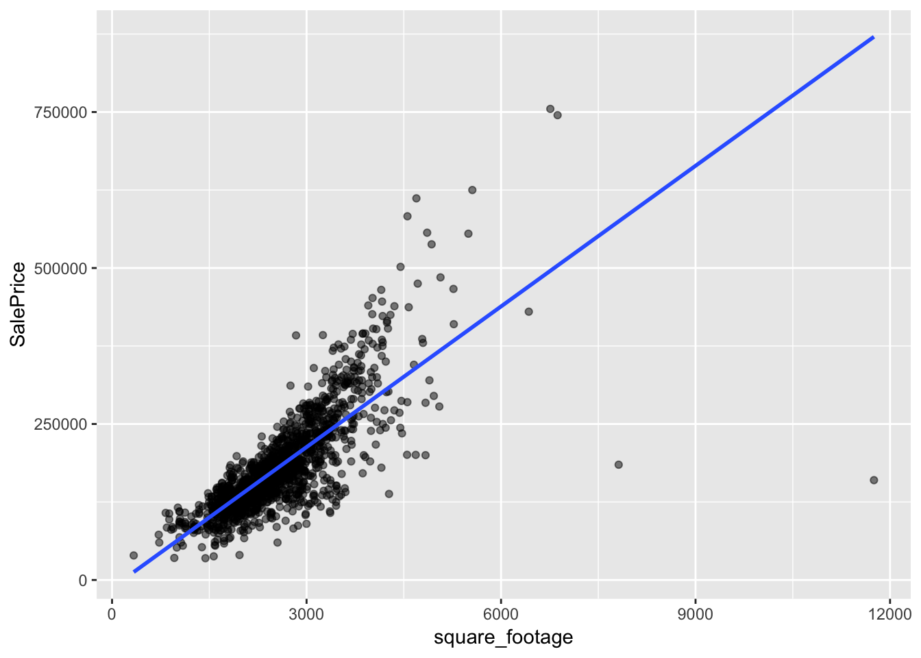
and here is the model that adds the categorical variable bathroom_count to the model. In this case that means adding another two lines to the graphs where each line has the same slope, but differing intercepts.
two_var_mod <- lm(SalePrice ~ square_footage + bathroom_count, data=housing_data)

# augment the model so that I can get .fitted values for the plot
aug_two_var_mod <- augment(two_var_mod)

ggplot(aug_two_var_mod, aes(square_footage, SalePrice, color=bathroom_count)) +
  geom_point(alpha=.5) +
  geom_line(aes(y=.fitted)) +
  facet_wrap(~bathroom_count)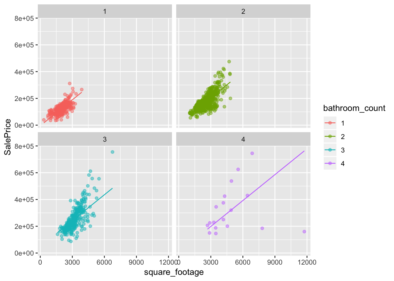
When multiplying explanatory variables together I get what is called an interaction term. The case of linear regression with one numeric variable and one categorical variable leads geometrically to multiple linear regression lines with differing slopes. This means that square_footage is somehow modulated by bathroom_count, this is logical since as the bathroom_count increases we would expect square_footage to increase as well.
interaction_mod <- lm(
  SalePrice ~ square_footage +
    bathroom_count +
    square_footage * bathroom_count,
    data=housing_data
  )

aug_interaction_mod <- augment(interaction_mod)

ggplot(aug_interaction_mod,
       aes(square_footage, SalePrice, color=bathroom_count)) +
  geom_point(alpha=.5) +
  geom_line(aes(y=.fitted)) +
  facet_wrap(~bathroom_count)
Which model is better?
As one measure of model fit, I can compare the adjusted R2 between the models to see which explains more of the total variation in the model. I use the adjusted R2 because it penalizes the use of additional varibles as opposed to R2 which always increases with the addition of more variables.
model_comparison <- data.frame(
  model =
  c(
    "single variable model",
    "two variable model",
    "model with interaction term"
  ),
  adj_r_squared =
  c(
    glance(single_var_mod)$adj.r.squared,
    glance(two_var_mod)$adj.r.squared,
    glance(interaction_mod)$adj.r.squared
  )
)

model_comparison %>%
  arrange(desc(adj_r_squared))
## model adj_r_squared
## 1 model with interaction term 0.6923468
## 2 two variable model 0.6487565
## 3 single variable model 0.6065174The highest adjusted R2 is given by the model with the interaction term followed by the two variable model, indicating that allowing both slopes and intercepts to differ leads to the better model.
Multiple numeric explanatory variables
I can add as many variables to linear models as we want, but the ability to visualize the model breaks down after 3 variables. I will extend my two variable model without interaction to include the square footage of the garage to compare the adjusted R2 to those computed previously.
aug_three_var_mod <- lm(
  SalePrice ~ square_footage + GarageArea + bathroom_count,
  data=housing_data
)

glance(aug_three_var_mod)$adj.r.squared
## [1] 0.6851754The adjusted R2 falls at 0.6851754, which is between the two variable model and the model with the interaction term that I put together.
Logistic regression
The other topic covered in the course is logistic regression, which models the probability of an event occurring given a binary response variable. Logistic regression is particularly nice for modeling probabilities because the model output will always be restricted to be between 0 and 1 on the probability scale. Logistic regression is part of a family of generalized linear models (GLMs) that use a link function to model a response in a linear fashion. For logistic regression the formula is given as
\[ log(\frac{p}{1-p}) = \beta_0 + \beta_1 * x_1 + \beta_2 * x_2 + ... + \beta_p * x_p \]
In the formula, p is what I am interested in and the link function is \(log(\frac{p}{1-p})\). I will run a logistic regression using the first data set that I found, here, which has three variables of interest to me: Age, EstimatedSalary, and the binary variable Purchased. In the first model I will only use Age as an explanatory variable and then will use both Age and EstimatedSalary as explanatory variables.
purchase_model_1 <- glm(Purchased ~ Age, family="binomial", data = ad_data)
purchase_model_2 <- glm(Purchased ~ Age + EstimatedSalary, family = "binomial", data = ad_data)

ggplot(purchase_model_1, aes(Age, Purchased)) +
  geom_jitter(height = .05, alpha = .5) +
  geom_smooth(method = "glm", se = FALSE, color = "blue",
              method.args = list(family="binomial"))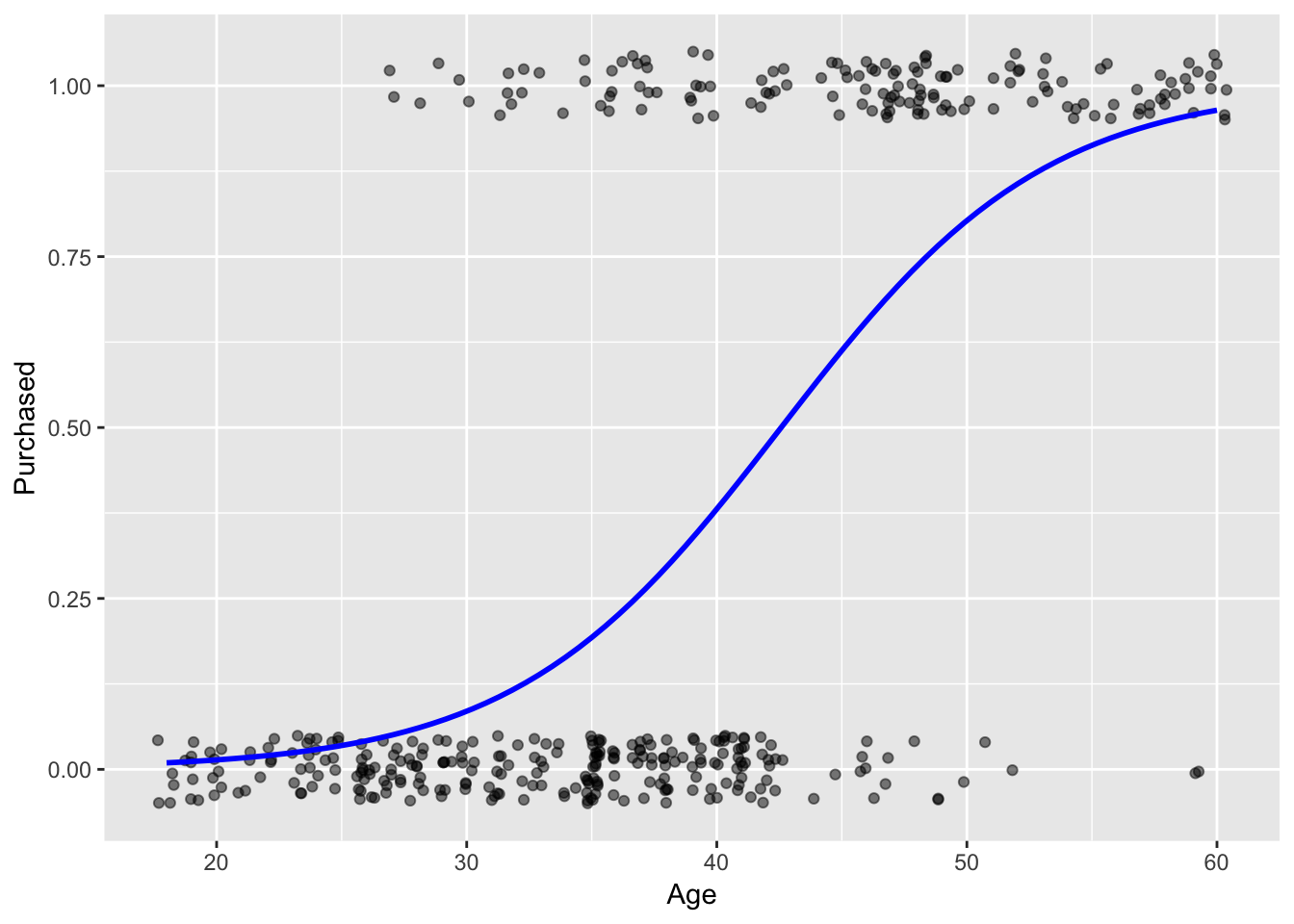
mean(ad_data$EstimatedSalary[ad_data$Age==40])## [1] 72200augment(purchase_model_1,
newdata = data.frame(Age = 50),
type.predict = "response")## # A tibble: 1 x 3
## Age .fitted .se.fit
## * <dbl> <dbl> <dbl>
## 1 50 0.803 0.0364augment(purchase_model_2,
newdata = data.frame(
Age = 50,
EstimatedSalary = mean(ad_data$EstimatedSalary[ad_data$Age==50])
),
type.predict = "response")## # A tibble: 1 x 4
## Age EstimatedSalary .fitted .se.fit
## * <dbl> <dbl> <dbl> <dbl>
## 1 50 47000 0.717 0.0530glance(purchase_model_1)## # A tibble: 1 x 7
## null.deviance df.null logLik AIC BIC deviance df.residual
## <dbl> <int> <dbl> <dbl> <dbl> <dbl> <int>
## 1 522. 399 -168. 340. 348. 336. 398glance(purchase_model_2)## # A tibble: 1 x 7
## null.deviance df.null logLik AIC BIC deviance df.residual
## <dbl> <int> <dbl> <dbl> <dbl> <dbl> <int>
## 1 522. 399 -139. 283. 295. 277. 397Based on the first model, a person aged 50 has a .80 chance of Purchase. Based on the second model, a person aged 50 with a salary of 47,000 has a .72 chance of Purchase. Given these two models, and a simple rounding method, we would predict a Purchase. The performance metrics seem to favor the second model over the first (higher logLik, lower AIC and BIC)
Conclusion
The course has given me a good basis for beginning with these models and the basics that I need to apply them. From here I need a lot more practice so that I can readily apply these methods when needed. I also plan to seek out more information on model evaluation when using multiple linear repression and logistic regression. The DataCamp course was well worth the effort and has much more content than I have applied here, including understanding the interpretation of coefficients under the different models, Simpson’s Paradox, visualizing models in three dimensions, and understanding the different scales of logistic regression.