I’ve finished the Introduction to machine learning with R course and wanted to write about the course and share my notes on the first couple of chapters.
Thoughts on the course as a whole
This course was longer than your typical DataCamp course but was well worth the extra time. I think I’ve been half consciously half subconsciously afraid to start machine learning for a while, thinking that I wasn’t ready for the abstract nature of the subject. This course however made the Machine Learning approachable. The broad concepts of all the techniques in the course:
- decision trees
- k-Nearest Neighbors
- regression
- k-Means
- hierarchical clustering
were easy to follow. I did have trouble with figuring out how ROC curves were built and why, for scree plots, the ratio of within sum of squares to total sum of squares always falls for an increasing number of clusters. The exercises related to those two topics felt a little plug and chug to me.
The instructors are very good, interesting, and have a lot of good hand movements (I probably rate hand gestures too highly).
Working through the course
While working through the first couple of chapters on the DataCamp site, I was using RStudio to half take notes and half dig deeper into some of the material that I found interesting. Keep in mind these are a student’s thoughts anything incorrect here is my doing.
Here are the packages used in what follows:
library(ggplot2)
library(dplyr)
library(tidyr)
What is Machine Learning?
Machine Learning at its core is the construction and use of algorithms to learn from data. The more data that we feed to the algorithms, the better the solutions that we get. Once we learn from the data we are working with we can generalize that algorithm to make predictions using newer data. The data is made up of “features” and “labels”, akin to “explanatory” and “response” variables in the statistical literature.
My first machine learning technique!
Upon starting the course, I was surprised to learn that the mysterious machine learning subject included regression, which I was already somewhat familiar with from statistics courses and from a DataCamp course on regression.
The goal of regression is to model a quantitative response as a linear function of predictors. \[ mpg \approx \beta_{0} + \beta_{1} \cdot wt \]
my_ML_model <- lm(mpg ~ wt, mtcars)

summary(my_ML_model)
##
## Call:
## lm(formula = mpg ~ wt, data = mtcars)
##
## Residuals:
## Min 1Q Median 3Q Max
## -4.5432 -2.3647 -0.1252 1.4096 6.8727
##
## Coefficients:
## Estimate Std. Error t value Pr(>|t|)
## (Intercept) 37.2851 1.8776 19.858 < 2e-16 ***
## wt -5.3445 0.5591 -9.559 1.29e-10 ***
## ---
## Signif. codes: 0 '***' 0.001 '**' 0.01 '*' 0.05 '.' 0.1 ' ' 1
##
## Residual standard error: 3.046 on 30 degrees of freedom
## Multiple R-squared: 0.7528, Adjusted R-squared: 0.7446
## F-statistic: 91.38 on 1 and 30 DF, p-value: 1.294e-10ggplot(mtcars, aes(wt, mpg)) +
geom_point() +
geom_smooth(method = "lm")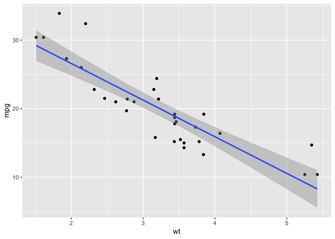
# a simple prediction
predict(my_ML_model, data.frame(wt = 4.5))
## 1
## 13.235Yes! did it.
More machine learning techniques!
Three common ML techniques include Classification, Regression, and Clustering.
Classification
The goal of classification is to predict the category of a new observation. An example that I’ve seen is the use of a dataset of pictures of both mops and dogs to predict which of the two the new picture represents.

But the techniques of classification don’t require the use of pictures, but instead enough feature data to place an observation into a group. A overly simple analogy comes to mind for me of an auto repair shop and how mechanics (good mechanics) can put a car problem into a category in their head based on the sound or smell of a car. Or maybe even how we have an idea about the size of a car by the sound it makes with the road without ever seeing it.
Clustering
The goal of clustering is to group similar objects together while minimizing the dissimilarities between groups. This sounds similar to classification for me, but I believe the difference is that we do not care beforehand which group an object belongs to, but rather that the clustering algorithm groups objects most effectively.
Supervised vs. Unsupervised learning
The machine learning models that need labeled data to work fall under the supervised learning category, so we can lump classification and regression in here. Unsupervised learning doesn’t require labeled observations, we can throw clustering in here.
Semi-Supervised Learning
Interestingly, we can combine supervised and unsupervised techniques. If I have only some of the data labeled, I can perform an unsupervised technique to assign labels based on my limited label information so that I am able to perform a supervised technique.
This sounded cool to me, so I tried to make up an example. Say that for a set of cars we have mpg, wt, and incomplete cylinder data. If we could use clustering on these observations, and if it happens that the observations fall neatly into the resulting groups, then I can assign the constituents of the cluster the label that is most representative of its group. To do this I am going to mimic the mtcars data set with some of the cylinder information removed.
set.seed(1)

my_cars <- data.frame(
  mpg = mtcars$mpg,
  wt = mtcars$wt,
  cyl = mtcars$cyl
)

# remove about 3/4 of the cyl data
to_remove <- rbinom(32, size = 1, prob = .25)
my_cars$cyl <- ifelse(to_remove == 1, mtcars$cyl, NA)

# did I do that right?
my_cars$cyl
## [1] NA NA NA 6 NA 6 8 NA NA NA NA NA NA NA 8 NA NA 4 NA 4 4 NA NA
## [24] NA NA NA NA NA 8 NA NA NAmean(!is.na(my_cars$cyl)) # around .25?## [1] 0.25cat("yes")## yes# peek at non labeled data in gray
ggplot(my_cars, aes(wt, mpg, col=as.factor(cyl))) +
geom_point()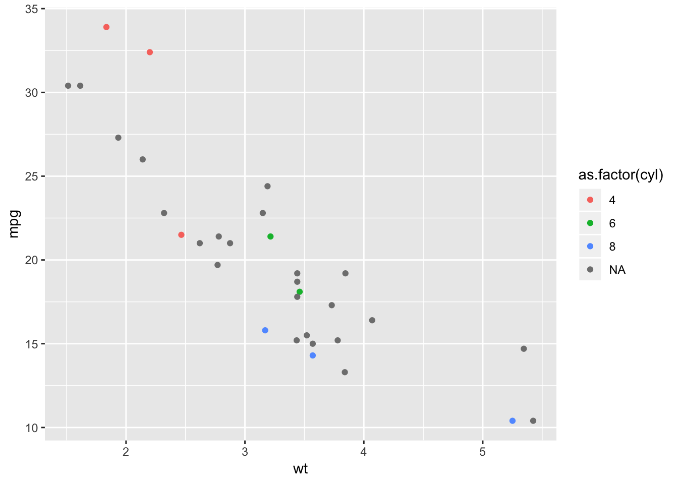
Now that I have my data set with missing cylinder information, I can apply k-means clustering to assign a cylinder count to each observation that is missing that label.
# set cluster count to the number of remaining clusters in the data set.
cluster_count <- length(unique(my_cars$cyl[!is.na(my_cars$cyl)]))

# apply k-means clustering
kmeans_my_cars <-
  kmeans(my_cars[, c("mpg", "wt")], cluster_count)

# how does the cylinder variable in my dataset fall into the clusters
table(my_cars$cyl, kmeans_my_cars$cluster)
##
## 1 2 3
## 4 0 1 2
## 6 0 2 0
## 8 3 0 0It looks like those with 4 cylinders got mostly assigned to cluster 3, those with 6 to 2, and those with 8 to 1. I’ll use this information to fill in the missing cylinder values in my data set.
# find the missing cyl values
missing_cyl <- which(is.na(my_cars$cyl))

#change cluster numbers to cylinder numbers
cyl_numbers <- case_when(
  kmeans_my_cars$cluster == 1 ~ 8,
  kmeans_my_cars$cluster == 2 ~ 6,
  kmeans_my_cars$cluster == 3 ~ 4,
  TRUE ~ NA_real_
)

# replace cylinder when cylinder is NA
my_cars$cyl[missing_cyl] <- cyl_numbers[missing_cyl]
Now that I’ve used clustering to give labels to the observations that had none, I’m going to compare to the mtcars data set.
# combine the two data sets so that I can facet them in the graph
df <- tibble(
  data_set = c("my_cars", "mtcars"),
  df_list = list(
    my_cars,
    mtcars[, c("mpg", "wt", "cyl")]
    )
  ) %>% unnest(df_list)

# data frame for centers of the clusters
centroids <- bind_cols(
  data_set = rep("my_cars", cluster_count),
  centroids = as.data.frame(kmeans_my_cars$centers)
)

ggplot(df, aes(wt, mpg, col=as.factor(cyl))) +
  geom_point() +
  geom_point(data=centroids, aes(wt, mpg), shape=15, color="black", size=2) +
  facet_wrap(~ data_set)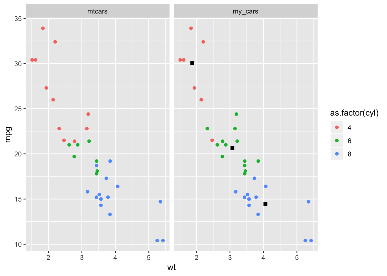
Not all the points match up, but the fact that they get close is pretty cool!
Now to handle the supervised portion of the semi-supervised approach. I can add a linear model to my new data set by cylinder.
df %>%
  filter(data_set == "my_cars") %>%
  ggplot(aes(wt, mpg, col=as.factor(cyl))) +
    geom_point() +
    geom_smooth(method = "lm", se = FALSE)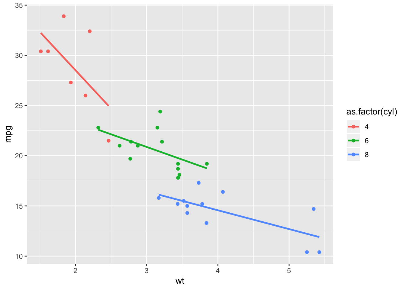
What makes a machine learning model useful?
The desirable traits of a model are that it is accurate, the calculations are not too computationally intensive for the task at hand, and that we can interpret the results.
Evaluating classification models
For classification, an important metric is the proportion of the time that a model makes the correct classification. But accuracy can be tricky, particularly with uncommon or very common events. With very uncommon events, like a meteorite landing in your house on a particular day, if you predict that it will never happen, then your accuracy will be through the roof. Even after a chance meteorite has done its damage, you’d still be very accurate.
The confusion matrix
The confusion matrix contains the counts of the number of times we correctly classify an object or event and the counts of the number of times we don’t. From this we can calculate the following ratios
- Accuracy: the number of correct predictions over the total number of predictions. How often am I right?
- Precision: the number of correct predictions for a group divided by the total number of times a prediction of that group was made. When I predicted this group, how often was I right about it?
- Recall: the number of correct predictions for a group divided by the total number in the group in actuality. When I predicted this group, how much of the group have I captured?
Evaluating regression models
One measure of accuracy when using regression models is the Root Mean Squared Error (RMSE). If I look back at the summary of the regression model that I put together at the beginning of my notes, I can see that the RMSE is 3.0458821. RMSE is meaningful when comparing it to the RMSE from another model of the same problem or when we have some idea of how small the error is intuitively.
#  See the third row from the bottom.
summary(my_ML_model)
##
## Call:
## lm(formula = mpg ~ wt, data = mtcars)
##
## Residuals:
## Min 1Q Median 3Q Max
## -4.5432 -2.3647 -0.1252 1.4096 6.8727
##
## Coefficients:
## Estimate Std. Error t value Pr(>|t|)
## (Intercept) 37.2851 1.8776 19.858 < 2e-16 ***
## wt -5.3445 0.5591 -9.559 1.29e-10 ***
## ---
## Signif. codes: 0 '***' 0.001 '**' 0.01 '*' 0.05 '.' 0.1 ' ' 1
##
## Residual standard error: 3.046 on 30 degrees of freedom
## Multiple R-squared: 0.7528, Adjusted R-squared: 0.7446
## F-statistic: 91.38 on 1 and 30 DF, p-value: 1.294e-10Evaluating clustering models
What you want most from clustering is at least conceptually simple. I want the differences within a cluster to be as small as possible while the differences between groups is as large as can be.
Here is an example of 4 sharpshooters named “A”, “B”, “C”, and “D”. “A” has the best within group similarity, followed closely by “B”, and “C”. “D” has atrocious within group similarity and causes the difference between groups to be much too small.
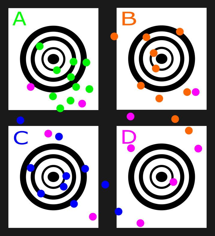
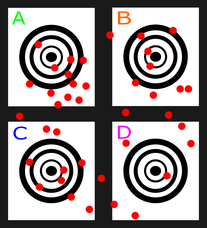
the problem with clustering here can be seen if I remove the differentiating colors. If this was done and I had to make a best guess on which shooter was which I would probably divide them up equally and pick the dots that were closest to each target center.
Testing and training
To maximize the predictive power of our models we break our data into training sets and test sets and base our performance measures on the predictions made using the test set. If a model that learns from a training set performs well on the test set, then a good model may be in the making. There is a trade-off when choosing the size of the testing and training sets though, I want the training set to be large enough to make a good model and the testing set to be large enough to produce meaningful performance measures.
Cross validation
I can split a data set into training and test sets many times using cross validation. If I was using three-fold validation I would construct three distinct breakups of the data into training and testing sets. For each fold, the model is trained on the training set and evaluated on the test set. We can use the performance metrics of each fold to better understand the performance of the model as a whole.
Error, overfitting, and underfitting
All models will have error and if it can be reduced then it should be. The error that I can’t do anything about is called irreducible and it is the product of the randomness within the system. Reducible error comes in the form of bias and variance.
- Bias is the difference between predicted and true values. Due to the complex nature of reality, bias will be higher the further away from that reality I get.
- Variance is the error due to fitting the training set too well. If I do that then the variation in results from one test set to another will be high.
As a machine learning algorithm gets more specific it picks up more and more noise and its variance increases, the model is becoming overfit. To make our models pick up less noise we have to make them less specific. But in the process of simplification we pick up less signal as well, thus moving us further from the truth, increasing bias, and towards underfitting the model. Models that are easier to explain are usually simpler and will have higher bias than those models that are more complex with higher variance.
Conclusion
These have been my notes on only the first two chapters. There is much more detail and subject matter in the course. My interest has been peaked and I am now excited to take additional courses on machine learning.